The periodic tables of algebraic geometry: curves and surfaces

Curves: Riemann

The first classification we look at will be of the simplest objects we can try to classify: curves, or one-dimensional varieties.

We have already seen an important recipe and some examples to describe curves: take a homogeneous polynomial \(f\in\mathbb{C}[x,y,z]\) of degree \(d\) and consider its zero locus \(\mathbb{V}(f)\subset\mathbb{P}^2(\mathbb{C})\). The pictures in Figures 3a and 3b really live in \(\mathbb{C}^2\), but e.g., for Figure 3a we can remedy this affine vs. projective discrepancy, replacing \(-y^2+x^3-2x\) by \(-y^2z+x^3-2xz^2\).

Can we describe all curves using a single homogeneous polynomial in 3 variables? In other words, is every curve a plane curve, living in \(\mathbb{P}^2(\mathbb{C})\)? No. But one can show that every curve is a space curve: it can be described by several polynomials in 4 variables, so that it is a curve living in \(\mathbb{P}^3(\mathbb{C})\).

But does this help in the classification of curves? Recall that we don’t want to classify polynomials, because those are only the tools to describe the curves. So we need to talk about things which are intrinsic to the geometry of a curve, independent of the realisation.

A discrete invariant

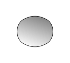
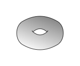
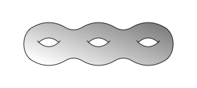
For this we can look at an algebraic curve as a so-called Riemann surface: because we work over the complex numbers, a topologist’s picture of a curve is really 2-dimensional. This is also how they were originally studied by Riemann in the 1850s. We end up with drawings as in Figures 4a, 4b and 4c. They correspond to plane curves of degree 2, 3 and 4 respectively. The obvious difference between these pictures is “the number of holes”. Mathematicians refer to this number as the genus.

It is similar to what a biologist would use to distinguish a giraffe from a fish: the former has 4 legs, the latter has none. Therefore they must be different in a meaningful sense, and the biologist will say they belong to different species (even though they are both animals).

So for now the “periodic table” of the classification of curves looks pretty bland: it is just the sequence of integers \(0,1,2,\ldots\) But biologists don’t stop classifying animals after having counted their legs, and neither will we after counting holes.

On a Riemann surface mathematicians study certain additional structure which allows us to speak about the curvature. This curvature is either \(+1\), \(0\) or \(-1\). The case of a sphere (as in Figure 4a) has positive curvature, the case of a torus (as in Figure 4b) has zero curvature (we say it is flat), and all other cases (e.g., Figure 4c) have negative curvature. Thus, there is an additional trichotomy into \(g=0\), \(g=1\) and \(g\geq 2\).

Continuous parametrisations

But this is still not the end of the classification of algebraic curves. We have described a Riemann surface of genus 1 using a homogeneous polynomial of degree 3. What happens if we start varying the coefficients of this polynomial? For example, what if instead of the homogeneous version \(y^2z=x^3-2xz^2\) of the equation in Figure 3a, we consider \(y^2z=x^3-3xz^2\)? We can show that they define “the same” curve: they are isomorphic.

But what if we consider \(y^2z=x^3-3xz^2+2z^3\) instead? Then we can actually show that the curves are different, even though the genus is 1 in both cases. For this we’d have to use something called the \(j\)-invariant: a number attached to every genus 1 curve. In the former case it is equal to 1728, in the latter it is 864 (quick word of warning: the \(j\)-invariant is not a count of anything, in general it can be any complex number). Thus to a trained algebraic geometer these are in fact different curves. Hence we can use parameters in our equations and get truly distinct answers. In our example changed the coefficient of \(z^3\) from \(0\) to \(2\), and we could in fact have considered all intermediate values (including complex numbers) to get all kinds of non-isomorphic curves of genus 1. They are usually referred to as elliptic curves, and they are an important tool in modern cryptography.

This continuous behavior is not something that happens in the periodic table of elements: you can’t move from hydrogen to helium by adding tiny fractions of neutrons, electrons and protons. The closest analogy in science is the Hertzsprung–Russell diagram, where you can vary the luminosity and temperature of a star continuously.

What about other degrees? Here the trichotomy into \(g=0\), \(g=1\) and \(g\geq 2\) comes back into play. We can show that for \(g=0\) there are no parameters possible (so there is a single curve of genus 0), whilst for \(g\geq 2\) there are in fact \(3g-3\) parameters (so there are many curves of genus \(g\), and describing them all in a suitable sense is an interesting problem). This result for \(g\geq 2\) is what Riemann obtained back in 1853, effectively introducing the notion of a “moduli space” to mathematics: a parameter space to describe all curves of a given genus.

More precisely, a moduli space is a new geometric object, that acts as a record-keeping device to describe a classification that involves continuous parameters. Every point in the moduli space corresponds to a certain element in the classification, and if we move a tiny bit in the moduli space we modify the element accordingly by a small amount to get a new element in the classification. If we move around in a different direction, we get another element in the classification.

This turns a classification of shapes into a new shape, and thus we can use all the tools from algebraic geometry to study it. Many questions about a classification can be phrased in terms of geometric properties of the moduli space, and mathematicians study moduli spaces of all kinds.

Smooth projective surfaces: Enriques

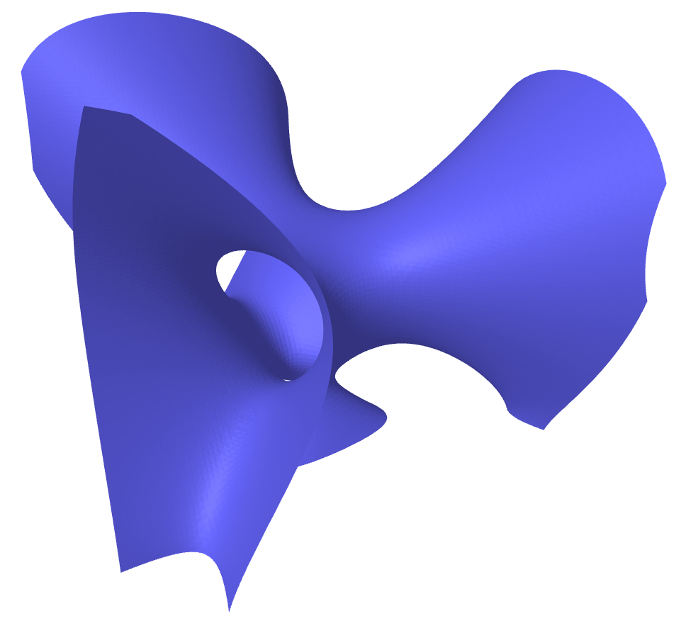
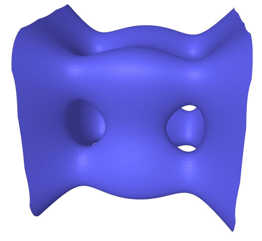
Going up one dimension we end up with surfaces. They have been at the forefront of algebraic geometry since the 19th century. The easiest algebraic surfaces we can produce are by taking a homogeneous polynomial in 4 variables, and consider \(\mathbb{V}(f)\) in \(\mathbb{P}^3(\mathbb{C})\). Because we are working over the complex numbers this would require a 4-dimensional drawing, which goes beyond what we can do here. But in Figures 5a and 5b we do what algebraic geometers often do: make a picture of an affine piece over the real numbers.

The classification of smooth projective surfaces is due to Enriques, as his life’s work, posthumously published in 1949. We will necessarily have to gloss over many details, but we will highlight some of its most interesting features. Without further mention we will classify minimal surfaces: every surface can be reduced to such a surface in a controlled way, and we know how to go back. Thus it suffices to classify these.

Trichotomy

Just like for Riemann surfaces we have a notion of curvature, introducing an important trichotomy between positive, flat and negative. With curves we had that positively curved case was the easiest, there being a unique such curve. For surfaces this is still the easiest case, but the uniqueness no longer holds: there are now 10 families of so-called del Pezzo surfaces, named after the mathematician who classified them in 1887. Some of these are unique in their family, for others there are continuous parameters.

If we consider a single homogeneous polynomial in 4 variables, the cases of degree \(d=1,2\) and \(3\) give rise to del Pezzo surfaces. In Figure 5a we have given an impression of an important cubic surface, where \(d=3\). The geometry of these del Pezzo surfaces is already rich enough to fill entire books— even though their classification is relatively straightforward— and their higher-dimensional analogues will be important for what follows.

What about the flat case, the 2-dimensional analogue of elliptic curves? There are now two distinct families. The closest analogue of elliptic curves are abelian surfaces. But there are also K3 surfaces, named so by Weil in 1958 after the recently climbed K2 mountain in the Himalayas, and the three mathematicians Kummer, Kähler, and Kodaira, who had been building the tools to study algebraic geometry and these surfaces in particular.

If we again consider a single homogeneous polynomial in 4 variables, the case \(d=4\) gives rise to a K3 surface, thus in Figure 5b we see an impression of an example. As with del Pezzo surfaces, their geometry is rich enough to fill entire volumes, and their higher-dimensional analogues will again be important for what follows.

The geography of surfaces: surfaces of general type

We now come to the analogue of curves of genus \(g\geq 2\). There are such curves for every value of \(g\), in fact there is an entire moduli space of dimension \(3g-3\) of them describing their classification.

Unlike for curves, a single integer is no longer enough to describe the crude classification of surfaces. Two important integers we can assign to a surface are the Chern numbers \(\mathrm{c}_1^2\) and \(\mathrm{c}_2\). For the genus we only had the inequality \(g\geq 0\) because we were counting something. For surfaces the situation is more complicated, and the possible values depend on the curvature. In the flat case \(\mathrm{c}_1^2=0\), whilst in the negatively curved case \(\mathrm{c}_1^2>0\). But what other conditions do we have?

We also have \(\mathrm{c}_2>0\), but more interesting we have that \(\mathrm{c}_1^2+\mathrm{c}_2\equiv0\bmod 12\). Besides this, there are two inequalities that need to be satisfied, the easier inequality to describe saying that \(\mathrm{c}_1^2\leq3\mathrm{c}_2\). In [figure:geography] we have drawn the “legal” values for sufficiently small Chern numbers. These conditions are similar to a law in biology saying that the number of legs on an animal is always even, but starfish are obvious counterexamples, so this particular universal biological law does not exist.

Now we have discussed necessary conditions on the Chern numbers. Are these also sufficient conditions, i.e., can we always find a surface with these allowed numbers? This leads to the problem of understanding the geography of surfaces, in particular those with negative curvature, which are called of general type,

We can already fill in two positions in our “atlas”: abelian and K3 surfaces have \(\mathrm{c}_2=0\) resp. \(24\). Next, if we take a homogeneous polynomial of degree 5, we get a quintic surface, for which \(\mathrm{c}_1^2=5\) and \(\mathrm{c}_2=55\). There are still many other legal values in Figure 6, and it is an interesting challenge to find a construction for a surface with given coordinates. We don’t know yet whether every pair of coordinates corresponds to a surface for instance, but luckily algebraic geometers know of many interesting and beautiful examples.

The important takeaway is that the classification of surfaces of general type is still an open problem, and it has been giving mathematicians enough material to work on for over a century.