The periodic tables of algebraic geometry: introduction

The periodic tables of algebraic geometry

To get a grip on the complexity of the world around us and the objects—such as animals, or chemical elements, or stars—appearing in it, we want to classify these objects. This allows us to describe the relationships, similarities, and differences between things we might be interested in, and thus further understand our world.

An early, and somewhat cruel, effort to understand a class of living creatures lead to lepidopterology: the study of butterflies and moths, most famously performed by sticking needles through them and displaying them in nice wooden cases, cf. Figure 1. From the 17th century onwards this was an important feature of humanity’s interest in biology, and it serves as a prime example of classification in biology. Another important example is Darwin’s description and classification of the beaks of the finches on the Galápagos islands, which led him to formulate the theory of evolution.

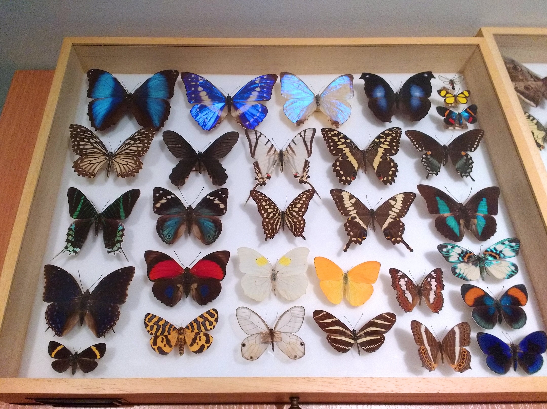
In this snapshot I want to introduce you to the idea that classification is an essential aspect of mathematics, just like it is for biology (and other sciences). The mathematical objects we will discuss are truly as pretty as the butterflies from Figure 1. And whilst in some cases it takes a bit of training as a mathematician to fully grasp their beauty, at least no living creatures need to be harmed to study them.

In §1 we will recall the periodic table of elements: an essential tool in modern chemistry, and the result of a lengthy classification effort. The organisation of elements like hydrogen, carbon, and uranium is similar to how mathematical objects are catalogued and have their properties described in a systematic way. Luckily, the study of these mathematical objects requires less interaction with dangerous chemicals.

An important feature is that these classification efforts are an ongoing process: when mathematicians complete one classification, they will move on to the next and more challenging one. That is why we will discuss periodic tables in algebraic geometry, going from the 19th to the 21st century, and from completely known settings to cutting-edge research.

1. The periodic table of elements

Every time one enters a chemistry classroom one is presented with a large poster, listing all the 118 known chemical elements together with their properties. This is the famous periodic table, and a very basic version is given in Figure 2. It lists elements like hydrogen, helium, and nitrogen in a specific shape which was essential for the development of chemistry in the 19th and 20th century, and continues to be used to explore and explain chemical elements.

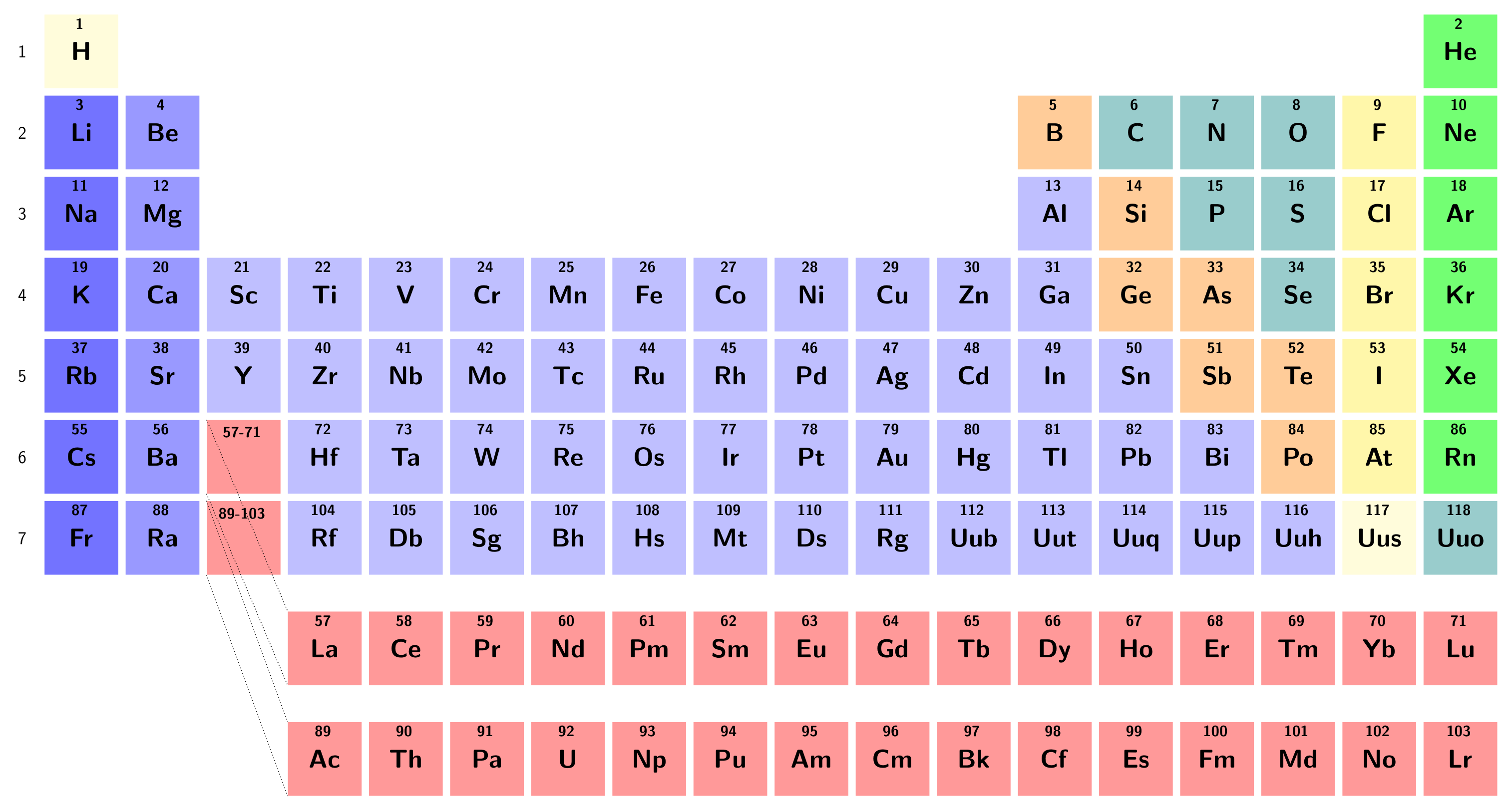
The name periodic table refers to an experimentally observed periodicity in the chemical behavior of elements: certain elements tend to exhibit similar behavior. For example the atomic radius has a periodicity: decreasing from left to right, and going up when going down in the table. In Figure 2, the inert noble gases are listed on the very right in light green, with the halogens as main building blocks for salts next to them, and the alkali metals in the first column all being soft and reactive metals. These observations are what chemists tried to formalise into a system. In 1869 Mendeleev catalogued the then-known elements in terms of atomic mass, obtaining the periodic table we now know.

Originally there were gaps in the table: elements that were predicted to exist, but which were not yet discovered. The periodicity of the periodic table also predicted some of the properties that these elements were required to have. For example, Mendeleev predicted the existence of an element with atomic mass \(\pm72.5\), a high melting point, and a gray color. This was element was subsequently found in 1887, and called germanium, in order to fill the gap which existed at position 32.

Invariants of elements

The periodic table in Figure 2 is a simplification of the periodic table as you usually see it. For space reasons we only list the chemical symbol and its atomic number. But usually a periodic table contains lots more data, such as the atomic weight, the melting and boiling point, the electron configuration, etc. There exists a beautiful interactive version too.

These are all examples of invariants of the objects being classified: properties of the chemical elements that do not change over time, and that do not depend on who measures them. By measuring invariants we can identify which chemical element we are looking at, and distinguish different elements. This is an important idea in mathematics too: mathematicians love to study invariants of objects, and then use them to distinguish between different objects.

Stars and the Hertzsprung–Russell diagram

In the first paragraph we also mentioned that one can try to classify the stars in the sky. To better understand an important aspect of classifications in mathematics we need to discuss how classifying stars is different from classifying chemical elements.

Astronomers observed that not all stars are equal: some are brighter than others (even when accounting for the distance), and some are hotter than others. Back in the early 1910s Hertzsprung and Russell made a plot of those two properties of stars, and they noticed that some types of stars are impossible. There are no super-bright cold stars, nor are there very faint hot stars. And there are many stars like our Sun: they all have roughly the same brightness and the same temperature. The interested reader is invited to read up more on the Hertzsprung–Russell diagram.

The main takeaway is that it is possible to vary the parameters of a star, subject to certain rules imposed by physics. This is a feature not present in the periodic table, but something similar will happen in mathematics, so one better keep this behavior in mind.

2. Classifications in algebraic geometry

We now turn to classifications in mathematics. One famous instance of such a result in mathematics is the Classification of Finite Simple Groups (CFSG). A group describes the symmetries of an object, and group theory is a fundamental subject in modern mathematics. Just like molecules are built using atoms, Jordan showed in 1870 that every finite group is built using simple groups.

The first (interesting) simple groups were already discovered by Galois in 1831, when he was studying solutions of polynomials of degree \(\geq 5\). The first example contains 60 elements. The last group to be discovered (in 1981) was the Monster group, and it has approximately \(8\cdot 10^{53}\) elements. Through a large effort of many mathematicians the CFSG was obtained, stating that all simple groups had been found in those 150 years. For more on this see, e.g., Searching for the Monster in the Trees and Symmetry and characters of finite groups in this very Snapshots series.

We will instead focus on classifications in algebraic geometry, because the author is an algebraic geometer and not a group theorist, and because the story of classifications in algebraic geometry is less well-known than the CFSG. Algebraic geometry is the study of shapes described by polynomial equations. The shapes we will be interested in are smooth projective varieties, defined over the complex numbers. Let us unpack what this means.

Smooth projective varieties

First of all, working over the complex numbers is a necessity to make things tractable, but it also makes it harder to make drawings. Usually we visualise the complex numbers as the complex plane, with one real axis and one imaginary axis. But from the point-of-view of an algebraic geometer the complex numbers are really a one-dimensional object! That is why an algebraic geometer will often draw an impression of an object when considered over the real numbers. More concretely, Figure 3a is what an algebraic geometer would draw when drawing a curve, whilst Figure 4b is what a complex geometer would think of, but they really are manifestations of the same object.

Now, what does it mean to describe a shape using polynomials? If \(f\in\mathbb{C}[x]\) is a polynomial, so \(f(x)=a_dx^d+a_{d-1}x^{d-1}+\dots+a_1x+a_0\), we define the variety associated to it as \[\mathbb{V}(f)=\{\alpha\in\mathbb{C}\mid f(\alpha)=0\},\] the set of zeroes of \(f\) in the complex plane. This set is always finite if the polynomial is not constant zero and consists of at most \(d\) points if it is not constant. Over the complex numbers it consists of exactly \(d\) points counted with multiplicities. In general we will consider a finite collection of polynomials in \(n\) variables \(f_1,\ldots,f_r\in\mathbb{C}[x_1,\ldots,x_n]\), and define \[\mathbb{V}(f_1,\ldots,f_r)=\{(\alpha_1,\ldots,\alpha_n)\in\mathbb{C}^n\mid \forall i=1,\ldots,r\colon f_i(\alpha_1,\ldots,\alpha_n)=0\},\] the set of points (inside the affine space \(\mathbb{C}^n\)), or zero locus, satisfying all polynomial equations simultaneously. These subsets are called affine varieties.

Instead of affine varieties we will be interested in projective varieties. In the affine plane two lines can be parallel, but this causes annoying situations in which we have to say that two distinct lines intersect in precisely one point unless they are parallel. That is why we extend our affine geometry: to make statements like the one on intersections of distinct lines more uniform, and get rid of the exceptions. In the projective world we have that our initial two parallel lines now intersect in a point at infinity, so any two distinct lines now always intersect.

For this we need to replace the affine space in which affine varieties live, by projective space \(\mathbb{P}^n(\mathbb{C})\). It is defined by considering the set \(\mathbb{C}^{n+1}\setminus\{(0,\ldots,0)\}\) of all points except the origin in the affine space one dimension up, up to the equivalence relation which says that \((\alpha_0,\ldots,\alpha_n)\sim(\beta_0,\ldots,\beta_n)\) if there exists some \(\lambda\in\mathbb{C}\setminus\{0\}\) such that \(\alpha_i=\lambda\beta_i\) for all \(i=0,\ldots,n\).

To work with projective varieties using polynomials, we will only consider homogeneous polynomials: a polynomial in which every term has the same degree. For example \(x^2+y^2+z^2\) is a homogeneous polynomial of degree 2, in 3 variables. The projective variety associated to a collection of homogeneous polynomials \(f_1,\ldots,f_r\in\mathbb{C}[x_0,\ldots,x_n]\) is \[\mathbb{V}(f_1,\ldots,f_r)=\{(\alpha_0,\ldots,\alpha_n)\in\mathbb{P}^n(\mathbb{C})\mid\forall i=1,\ldots,r\colon f_i(\alpha_0,\ldots,\alpha_n)=0\}.\] This is well-defined because we restricted our attention to homogeneous polynomials, so that asking whether a polynomial is (non-)zero is independent of the scaling in the equivalence relation. The example \(x^2+y^2+z^2\) thus defines a curve in \(\mathbb{P}^2(\mathbb{C})\)—a conic—corresponding to Figure 4a.

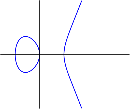
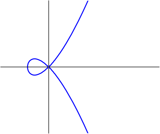
The final ingredient in order to describe the objects we are interested in is smoothness. This is best explained through an example: consider the following degree 3 polynomials \[\begin{aligned} f&=-y^2+x^3-2x \\ g&=-y^2+x^3+x^2 \end{aligned}\] describing affine curves living in \(\mathbb{C}^2\). If we draw these curves inside \(\mathbb{R}^2\subset\mathbb{C}^2\) we get the pictures as in Figures 3a and 3b. We immediately see that on the right there is something funny happening at the origin: there is a singularity. For more on singularities we refer to another Snapshot: Swallowtail on the shore.

Classifying smooth projective varieties?

In what follows next we discuss examples of classifications of smooth projective varieties. This will illustrate how the life of an algebraic geometer can be very similar to that of someone sticking needles through unsuspecting butterflies, or that of an experimental chemist inhaling noxious fumes in order to isolate an unknown chemical element.

Before we embark on our journey we need to point out that to an algebraic geometer classification can mean different things. Certainly, we are not just classifying polynomials, rather we are interested in classifying varieties independently of their realisation. This gives rise to classification we will mostly be talking about: that of varieties up to isomorphism, i.e. up to their realisation inside some projective space.

It turns out that already in dimension 2 this becomes impossible, so that we will only try to classify certain well-chosen objects. There is an entire branch of algebraic geometry, called birational geometry, devoted to understanding the precise relationships between smooth projective varieties which are different but nevertheless almost the same: we say that they are birational, but we will not discuss this further.