Howto: Draw algebraic curves using PGF/TikZ

Introduction

As one could deduce from my previous posts, I was trying to draw algebraic curves directly in LaTeX using PGF/TikZ and gnuplot. I'll present a short overview of how one can do this, hoping it will get as popular as my post on direct and inverse limits. Which is according to Wordpress' statistics good for one daily search hit.

So, what is an algebraic curve? For an extensive overview, I refer you to the Wikipedia article about them. In this post, it just boils down to an implicit function in 2 variables over the real field. That is, just take any polynomial $F\in\mathbb{R}[X,Y]$

and set it equal to zero. In general it is far more abstract, as can be seen in the Wikipedia article, but we're drawing plane algebraic curves, not n-dimensional hypersurfaces over exotic fields. To give an example, take $F(X,Y)=Y^2-X^3+X=0$

for now, this is the curve (even more, this is an elliptic curve) we'll be using in our examples. It corresponds to the a=-1, b=0 cell in the matrix of examples.

The set-up

We'll be using PGF/TikZ, the most awesome LaTeX package since the invention of the boiled water. Apart from maybe microtype. Anyway, to see what it can do I refer you to TeXample, a nice overview of the amazing stuff it can do. What it so far hasn't been doing is drawing algebraic curves. But we're about to change this!

Apart from PGF/TikZ, we'll need gnuplot, a tool for drawing plots (as its name suggests) and luckily for us: tightly integrated in PGF/TikZ. In case you're using Linux, it should only be a sudo apt-get install gnuplot (or similar) away. If you're using Windows, I'm afraid you'll have to figure out how to install and use it yourself.

Howto

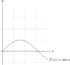
PGF/TikZ cannot draw implicit functions. Actually, it can only draw lines, splines and variations thereupon, as far as I know. But it can pass functions to gnuplot which then calculates the coordinates of enough points to provide a nice result. Let's draw a sine for example.

I've modified this example at TeXample (and snippet from the manual) a bit resulting in this code

\begin{tikzpicture}[domain=0:4]
  \draw[very thin,color=gray] (-0.1,-1.1) grid (3.9,3.9);
  \draw[->] (-0.2,0) -- (4.2,0) node[right] {$x$};
  \draw[->] (0,-1.2) -- (0,4.2) node[above] {$y$};
  \draw plot[id=sin] function{sin(x)} node[right] {$f(x) = \sin x$};
\end{tikzpicture}

which produces

So, let's pass our desired algebraic curve to gnuplot!

But gnuplot doesn't support implicit functions. So it's not possible to draw them. Wait? Why do you use it then? Because we can draw them by cheating a little. This is explained at their website. So we know how to draw them in gnuplot. How can we use that output?

This is where raw gnuplot comes to rescue. You basically feed gnuplot to the program and it outputs a .table file containing the necessary coordinates. So we end up with:

\begin{tikzpicture}
  \draw[very thin,color=gray] (-1.9,-3.9) grid (3.9,3.9);
  \draw[->] (-2,0) -- (4.2,0) node[right] {$x$};
  \draw[->] (0,-4.2) -- (0,4.2) node[above] {$y$};
  \draw plot[id=curve, raw gnuplot, smooth] function{
    f(x,y) = y**2 - x**3 + x;
    set xrange [-4:4];
    set yrange [-4:4];
    set view 0,0;
    set isosample 1000,1000;
    set table;
    set size square;
    set cont base;
    set cntrparam levels incre 0,0.1,0;
    unset surface;
    splot f(x,y)
  };
\end{tikzpicture}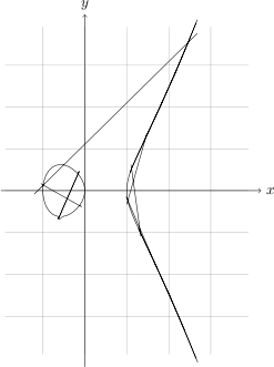

Not quite what we were expecting, don't you think? But there is an easy solution. First we observe that the .table file contains different segments. Apparently, the calculation of the intersection of the surface and the z=0 plane is not that accurate, which results in discontinuities and the segments are not placed in order. PGF/TikZ on the other hand is not aware of any segments and just connects them. Resulting in a cat's cradle of lines.

Now comes the hackish part. In /texmf/tex/generic/pgf/modules/pgfmoduleplot.code.tex, the definition of \def\pgf@readxyfile should read

\def\pgf@readxyfile{%
  \read1 to \pgf@temp%
  \let\par=\pgf@savedpar%
  \edef\pgf@temp{\pgf@temp}%
  \ifx\pgf@temp\pgfutil@empty%
  \else\ifx\pgf@temp\pgf@partext%
    \pgfplotstreamstart%
    \pgfplotstreamend%
  \else%
    \expandafter\pgf@parsexyline\pgf@temp\pgf@stop%
  \fi\fi%
  \ifeof1\else\expandafter\pgf@readxyfile\fi%
}

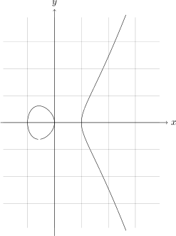
Much better, don't you think? The small gap at the bottom is due to my gnuplot 4.2 installation, in gnuplot 4.4 this is fixed (as shown by experiments on another computer) but I haven't yet updated mine.

Any questions?